Asymmetric loss for power duration models
Most applications of power duration models apply least squares regression to find the best fit through your data. This seems reasonable: take your best efforts at different durations, fit a curve, and voilà, you have a model of your capabilities.
But there’s a fundamental problem: least squares regression assumes errors in the data are symmetrical, and mean-max data absolutely does not behave that way.
What mean-max data really is
Mean-max curves represent your best efforts across different durations across a window of time, for example 90 days. In cycling or running, these curves show the highest average power, speed, or pace you’ve sustained for 1 minute, 5 minutes, 20 minutes, and so on.
Here’s the crucial distinction: mean-max data is fundamentally mixed in nature:
- Some points represent true maximal efforts: all-out time trials, race finishes, or structured tests where you gave everything.
- Many points are submaximal: pacing strategies, accumulated fatigue, poor conditions, or simply efforts where you didn’t need to go all-out.
The asymmetry problem
Think about what these data points actually mean:
- When your model underpredicts (says you can’t sustain power you’ve already achieved): This is definitely wrong. You have proof you can do better than the model suggests.
- When your model overpredicts (says you can sustain more than your recorded best): This might be right. That recorded “best” might not have been a true maximal effort.
The asymmetry is clear: underprediction is a definite error, while overprediction is only a potential error.
Why least-squares fails
Standard least-squares regression treats both types of errors equally. It “splits the difference,” minimizing the sum of squared residuals regardless of whether the model over- or under-predicts your proven performance.
Visualize your power curve with a least-squares fit. Notice how the line often passes below some of your data points? The model is literally telling you that you’re incapable of efforts you’ve already completed. Those regions below your proven performance represent physiologically impossible predictions.
This happens because least-squares allows underfitting of proven performance in exchange for avoiding overfitting of potentially submaximal data points.
The mathematical fix: asymmetric cost functions
The solution is to use asymmetric loss functions that penalize different types of errors differently:
- Underprediction errors: penalized heavily (quadratic, exponential, or other aggressive penalties)
- Overprediction errors: penalized lightly (linear, capped, or minimal penalties)
This approach draws from quantile regression and one-sided loss functions like hinge loss or pinball loss. Instead of finding the line that minimizes average error, we find the line that respects our proven capabilities while ignoring conservative estimates where data might be submaximal.
Cross-domain example: energy load forecasting
Consider energy load forecasting: if you underestimate electricity demand, you risk blackouts: A catastrophic failure with severe consequences for the grid. If you overestimate demand, you’ll have excess capacity, which is costly but manageable without system failure.
Similarly, if your power duration model underestimates what you can sustain, that’s definitely wrong and you have the data to prove it. If it overestimates, you might simply have not done a maximal effort for that duration.
Concrete example with power data
Let’s say your mean-max data shows:
- 2-minute best: 500W (maximal)
- 5-minute best: 380W (sub/near-maximal)
- 20-minute best: 350W (maximal)
Fitting the 2-parameter critical power model to these points using regular least-squares and an asymmetric loss function yields these results (see also plot below):
| Duration [min] | mean-max [W] | least squares [W] | asymmetric [W] |
|---|---|---|---|
| 2 | 500 | 496 | 499 |
| 5 | 380 | 393 | 399 |
| 20 | 350 | 341 | 349 |
(The code for this example is available here. Run it in an interactive browser sandbox at SweatStack.run.)
The asymmetric loss function forces the model to never predict below your proven performance.
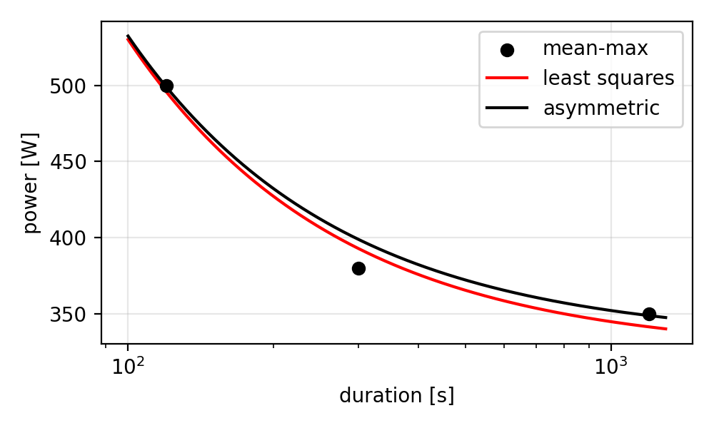
The result is that instead of underpredicting 9W at 20 minutes, we’re now overpredicting by 19W at 5 minutes, producing a more realistic critical power model that respects demonstrated capabilities.
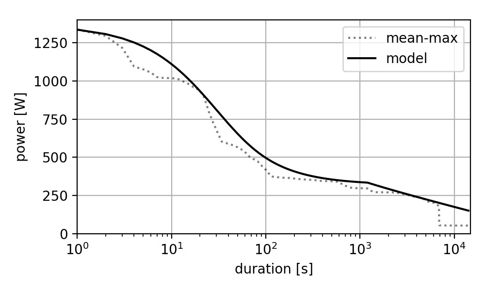
The same approach can be extended to other power duration models (such as the OmPD model) on more detailed mean-max data, showing the same effect of tightly fitting around proven maximal efforts while ignoring submaximal efforts:
Discussion
While asymmetric loss functions offer clear advantages for power duration modeling, several practical considerations deserve attention.
Data dependency: This approach assumes that the mean-max data contains enough maximal efforts across the range of durations you are fitting the model to. The defintion of “enough” is subjective though, and also depends on the chosen model and tuning of the asymmetric loss function.
Model dependency: This approach assumes your underlying power duration model (critical power, OmPD, etc.) accurately captures the relationship between power and duration. If the model structure itself is flawed, this approach can still lead to underpredictions or unrealistic overpredictions.
Parameter tuning: The asymmetric loss function requires careful calibration. Too aggressive penalties on underprediction can force unrealistic overpredictions.
When to use traditional methods: Least-squares remains appropriate when working with controlled laboratory data where all efforts are truly maximal. For exploratory analysis or when model uncertainty is high, symmetric approaches may be more suitable.
Validation strategies: Standard cross-validation cannot be applied to asymmetric regression models, since they’re designed for symmetric errors. Instead, validate against known maximal efforts or structured tests where true performance limits are established.
Conclusion
Mean-max data has a built-in asymmetry that least-squares regression simply cannot handle appropriately. When your model predicts you’re weaker than your data, it’s not just mathematically questionable, it violates basic physiological constraints.
The mathematics behind asymmetric loss functions aren’t complex. Most optimization libraries support custom cost functions. The conceptual shift, however, is crucial: our models should respect what athletes have proven they can do while remaining appropriately conservative about untested performance.
I am working on an implementation of this approach in SweatStack. It’s already available for testing here. Please give it a try and let me know what you think!