Resampling discontinuous power to 1 Hz
tl;dr: Averaging rowing power over each second really is chaos: off by about 110% at 22 spm, against about 4% for cycling. But average per stroke first and then go to 1 Hz, and almost nothing is lost. A time-weighted average of the strokes keeps total work exactly right and everything else within about half a percent. Store each stroke’s own power next to it, and even its last downside is gone.
Cycling power is stored at 1 Hz. Rowing power is mostly stored once per stroke. A discussion on the Rowing Data Standard made me wonder: both sports produce power discontinuously, so why does 1 Hz work fine for cycling? And what do you lose if you resample rowing power to 1 Hz?
These are my notes from trying to find out.
Why bother with 1 Hz
Why resample at all, instead of keeping the data the way it was recorded?
- Most power analysis assumes one sample per second: mean-max, normalised power, time in zones, training load, W’ balance. A 5 min mean-max is the best rolling average over 300 samples.
- With one sample per stroke, all of these need time weighting, and often resampling anyway: a power-duration curve needs power over 180 s, not 181.3 s. That’s easy to get wrong.
- Every consumer of a file could resample on their own. But that’s what standards like FIT (and the Rowing Data Standard on top of it) are for: so not every developer has to do the same work, solves the same problem slightly differently, and ends up with a different mean-max curve.
Two places where information gets lost
- Instantaneous → one value per revolution or stroke: the shape within the stroke is lost: peak power, timing, force build-up.
- One value per revolution or stroke → 1 Hz: the link to the stroke, exact timing, maybe some stroke-to-stroke variation.
Peak power is gone after step 1, whatever you do next. This post is mostly about step 2.
The data
To see what happens within a stroke, I need power at a much higher rate than once per second:
- Cycling: a ride on a Wattbike, which records pedal force at 100 Hz. Written by the Wattbike to a .WSE file and reverse-engineerd by https://wattbike-wse-viewer.pages.sweatstack.dev/.
- Rowing: a Concept2 rowing machine. Its monitor (the PM5) sends a force curve for every stroke, plus drive length, drive time and work. I recorded these over USB.
Both give force, not power. Power is force × speed, and neither records speed within a stroke, so I assume it’s constant:
- Cycling: pedal speed from the duration of each half revolution. Averaged per revolution, this matches the Wattbike’s own power within 0.4 W.
- Rowing: handle speed = drive length ÷ drive time, zero during the recovery. Each stroke is scaled to the PM5’s work per stroke.
Not the true instantaneous power, but “actual enough” for what matters here: when power is on, and for how long.
Why cycling gets away with it
Step 1 explained above is optional: you can also average instantaneous power over each second. In rowing that gives the “chaos” from the discussion. In cycling it works fine. Why?
1 Hz can only represent changes slower than 0.5 Hz, the Nyquist frequency (half the sample rate).
- Cycling: at 90 rpm there are 3 downstrokes per second, two per revolution. Power rises and falls much faster than 0.5 Hz, so a 1 s average smooths it out.
- Rowing: 20–36 spm is 0.33–0.6 strokes per second, right at the limit. One second catches mostly drive, the next mostly recovery.
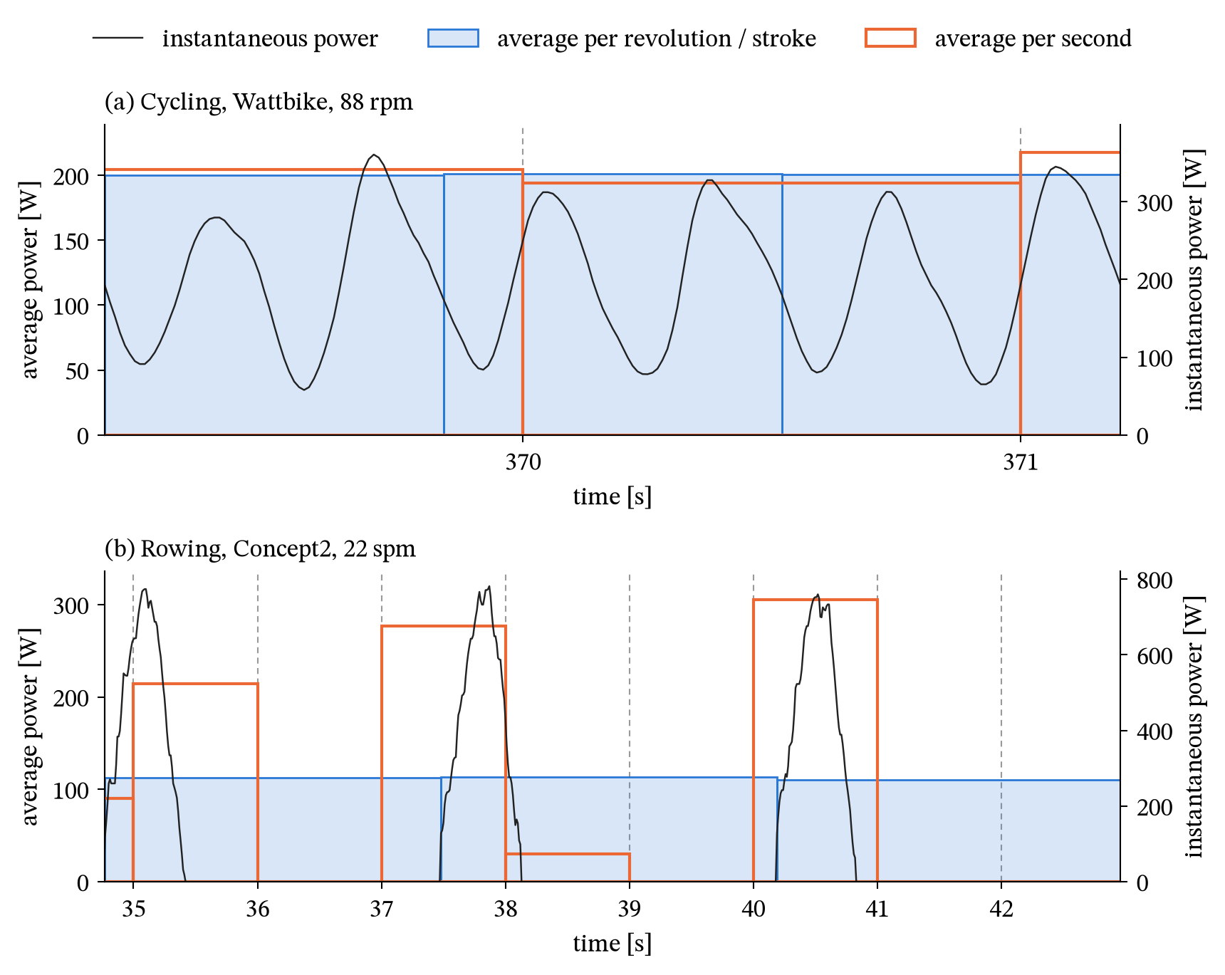
Real recordings. (script, data extraction, data: cycling, rowing)
So for rowing: average per stroke first, then go to 1 Hz. The question is how.
Six ways to get to 1 Hz
| Method | Note | |
|---|---|---|
| A | Average each second of instantaneous power | The “chaos” baseline |
| B | Hold the last completed stroke | What the Concept2 monitor shows |
| C | Give each second the stroke it falls in | |
| D | Time-weighted average of the strokes in the second | Total work exactly right |
| E | Interpolate linearly between strokes | |
| F | Average the strokes that ended in the second | Identical to B below 60 spm |
B to F only use what a per-stroke file holds: start, end and average power of each stroke. F is how you’d compute power from ANT+ data (accumulated power ÷ event count). Below 60 spm at most one stroke ends per second, so for rowing F is the same as B, and I’ll leave it out below.
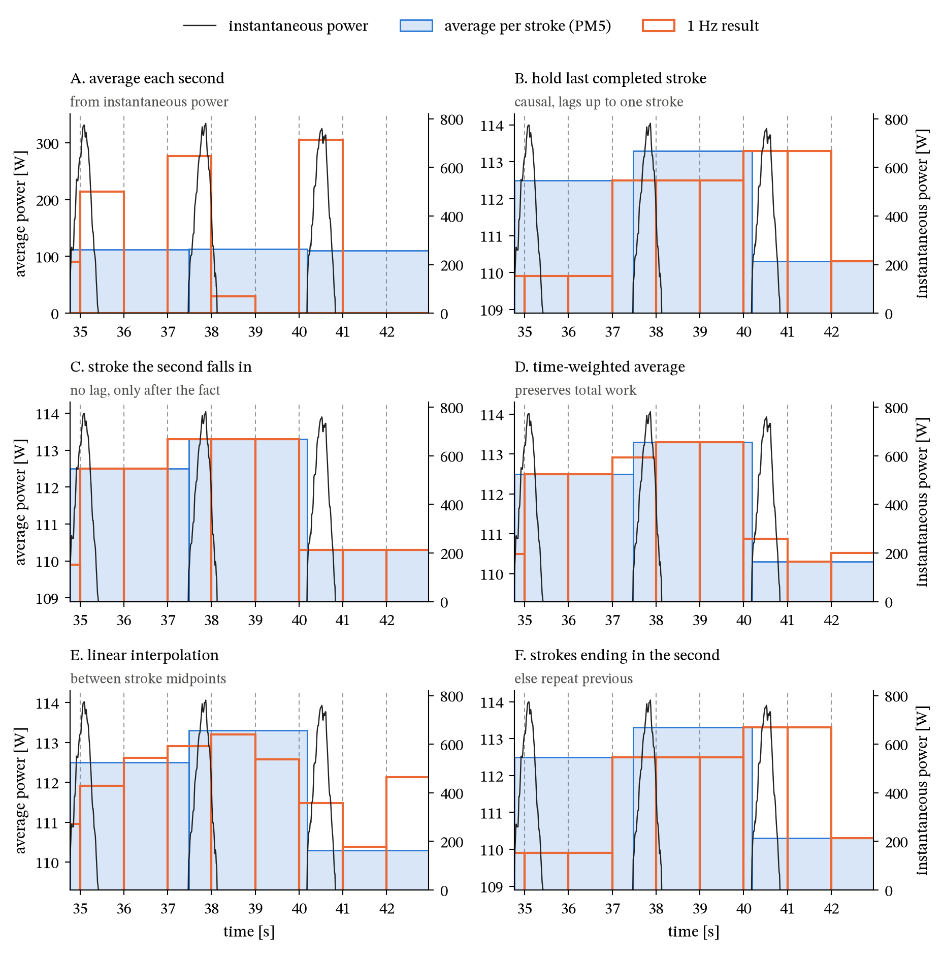
The same three strokes as above. Note the different y-axes: A spans 0 to 300 W, B to F only 110 to 114 W. (script, data)
On steady strokes B to F are within 3 W of each other. They differ in timing:
- B is a stroke behind: a second shows the previous stroke until the current one is done.
- C follows the strokes, rounded to whole seconds.
- D blends two strokes in the seconds where they meet. E blends everywhere.
Whether that matters shows once the pace changes.
Setup
- Real rowing: 209 strokes in 14 pieces. All easy rowing (100–120 W, ~22 spm): fine for stroke-level questions, too short and easy for the rest.
- Assembled rowing session: 34 min built from those real strokes: warm-up, 3 × 4 min at 28 spm and 230 W, 4 × 30 s sprints at 34 spm and 380 W, easy rowing in between. 20 versions with different strokes and timing.
- Real cycling: a 16 min Wattbike session, 1361 revolutions.
The reference (“ground truth”) is each stroke’s power held over that stroke’s duration: what rowers mean by power, and what a per-stroke file holds. 1 Hz values are rounded to whole watts, as FIT stores them.
(analysis.py produces every number below, extract_sessions.py gets the strokes out of the recordings, results.json has all the numbers.)
Results
1. Is the chaos real at every stroke rate?
The figure above shows a few strokes at one stroke rate. Does averaging each second (A) go wrong at every rate, and does cycling get away with it at every cadence? For every stroke rate from 16 to 45 spm and every cadence from 50 to 130 rpm, I simulated 5 min at a constant 200 W and measured how far each 1 Hz value lands from the actual power.
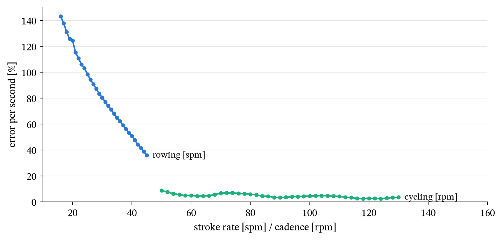
- Rowing: off by 111% at 22 spm, 81% at 30 spm, still 39% at 44 spm.
- Cycling: 2.5–9% at any cadence, 3.4% at 90 rpm.
The more strokes fit in a second, the better a 1 s average works. Rowing never has enough.
2. Do work, mean-max and normalised power come out right?
These are the numbers people actually use. I weigh total work the most: it’s what kilojoules, calories and training load build on, and if a file has both per-stroke and 1 Hz power, both should add up to the same work.
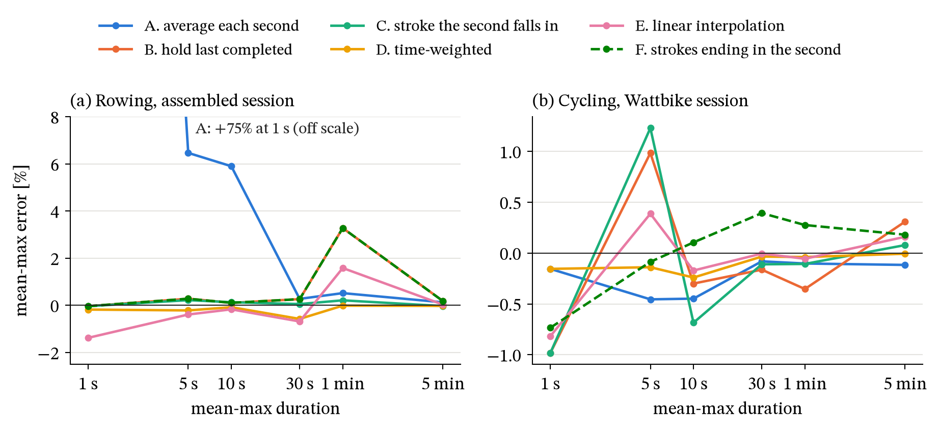
F is dashed because it’s identical to B for rowing.
Rowing, assembled session, error vs the reference:
| Work | 1 s | 5 s | 1 min | NP | |
|---|---|---|---|---|---|
| A. average each second | 0.0% | +75% | +6.5% | +0.5% | 0.0% |
| B. hold last completed | +0.7% | 0.0% | +0.3% | +3.3% | +1.0% |
| C. stroke the second falls in | 0.0% | 0.0% | +0.2% | +0.2% | 0.0% |
| D. time-weighted | 0.0% | −0.2% | −0.2% | 0.0% | 0.0% |
| E. linear interpolation | +0.4% | −1.4% | −0.4% | +1.6% | +0.5% |
- A inflates short efforts: your best 1 s is just the best-aligned drive.
- B overestimates work and 1 min power when the pace changes: each stroke’s power is shown during the next stroke, so going from a sprint to easy rowing stretches the last hard stroke.
- D gets work exactly right, in every session. C is off by at most 0.2%.
- Cycling: all methods within 1.2% on mean-max. Work is 1.4–2.0% high for B, E and F, exact for D.
3. Can you get the strokes back?
The main objection to 1 Hz: you lose the link to the stroke. FIT has a field for that, total_cycles: the number of strokes so far, stored with every 1 Hz record. With it, every stroke’s power can be read back from the 1 Hz data:
- B and C: every stroke back exactly, at every rate tested.
- D: 100% at 22 spm, 98% with the 34 spm sprints. D needs a second that falls entirely within one stroke, and short strokes don’t always have one.
- E: a third or less exact. A: practically none.
Without total_cycles you only see a stroke where the value changes, and 3–4% of the strokes disappear because two strokes in a row had the same power in whole watts. So store total_cycles.
4. Live, or after the fact?
A stroke’s power is only known once the stroke is over. That decides when each method can write a second:
- Live: the value is written at the end of every second. That’s what a screen does, or an app that streams power while you row. Only B can do this: it only uses strokes that are already over. The price: it runs about 2 s behind.
- After the fact: the value is written once the strokes it needs are over. C and D have to wait for the current stroke to finish: at most 2.4 and 2.8 s at 22 spm. E waits for the next stroke as well.
In practice a file never needs to be live, not even one recorded during the session. A recorder can keep the last few seconds in memory and write each second once its stroke is over. Nobody notices a file being three seconds behind. So:
- Screen or live stream: B, as the Concept2 monitor already does.
- File: C or D.
Conclusion
For rowing files, D is probably the way to go: total work exactly right, mean-max and normalised power within about half a percent, and with total_cycles nearly every stroke can be read back.
D has one weakness left: in the second where two strokes meet, its value is a blend of both, so not every 1 Hz value is a real stroke’s power. That’s solved by storing each second’s stroke power next to it, as a separate average stroke power field (method C). Then every time-based tool gets power that adds up to the right work, every stroke can be read back exactly, and total_cycles links the two. Nothing the comparison above found is lost. What’s left is the shape within the stroke, and that needs the per-stroke data and force curves anyway.
So the question for the Rowing Data Standard isn’t per-stroke or 1 Hz. Per-stroke data stays. The question is whether a few extra fields per second are worth it, so that every time-based tool can read rowing files without solving this again.
Caveats: the real rowing data is short and easy, the hard session is assembled from those strokes, and instantaneous power is derived from force rather than measured. A long, hard, real session is the next thing to try.