Same model, different regression
There are different ways to fit the 2-parameter CP model: You can transform the data, change what you’re optimizing, or use different regression techniques. My recent post about asymmetric loss is one example of this. But as a result of a discussion on Bluesky, I realized I didn’t have a good intuitive understanding of how some of these approaches actually work and what the differences are between them.
So I decided to dig in and implement some of these approaches to see how (if) they behave.
The basic model
The 2-parameter CP model is simple:
\[ \begin{equation} P = W'/t + CP \end{equation} \]Where:
- \(P\) is power output
- \(t\) is duration
- \(CP\) is Critical Power (the horizontal asymptote)
- \(W'\) is W-prime (the finite work capacity above CP)
This hyperbolic equation describes how power output decreases with duration.
My mean-max data
Let me start with my own cycling data from the past 6 months:
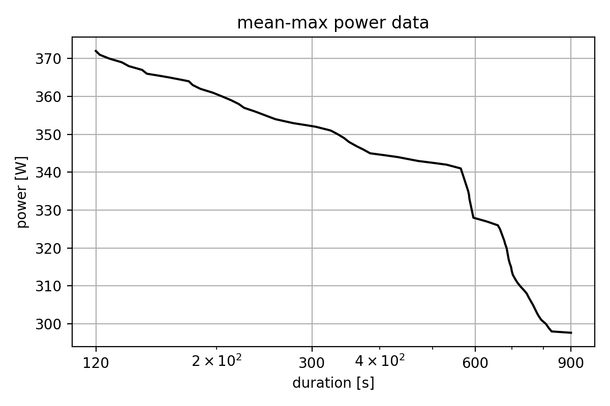
This is the typical mean-max curve: Highest average power I could sustain for each duration, plotted on a log scale. Now let’s see how different fitting approaches work with this data.
Three ways to fit the same model
1. Power-Duration: The direct approach
The most straightforward way is to directly fit \(P = W'/t + CP\) using non-linear least squares. This is what most software does: You give it the equation and it finds the \(CP\) and \(W'\) values that minimize the squared errors between predicted and actual power.
2. Work-Duration: Transform to work space
Here’s where it gets interesting. If I multiply both sides of the equation by duration:
- \(P * t = W' + CP * t\)
- \(W = W' + CP * t\)
Now I have work on the left and a simple linear equation: I can use linear regression to fit \(W = CP * t + W'\) where the slope is \(CP\) and the intercept is \(W'\).
3. Power-1/Duration: Linearize the hyperbola
Another transformation: the original equation \(P = W'/t + CP\) is actually linear if I plot \(P\) against \(1/t\):
- \(P = W' * (1/t) + CP\)
This is a straight line where the slope is W’ and the intercept is CP. Again, I can use simple linear regression.
Visualizing the different approaches
Here’s what the data and fitted model of each approach look like in its “natural” space:
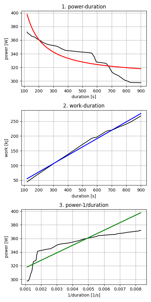
The first plot shows the traditional power vs duration view. The second shows how the relationship becomes linear when we transform to work space. The third shows the linearization when plotting against 1/duration.
Do they give the same answer?
This was the key question for me. In theory, they should all give the same CP and W’ values since they’re fitting the same underlying model on the same data, but I was expecting some differences. Let’s check the fitted model parameters:
| Method | CP [W] | W’ [J] |
|---|---|---|
| Power-Duration | 306 | 11027 |
| Work-Duration | 283 | 21291 |
| Power-1/Duration | 306 | 11027 |
Interesting! The first and third approaches give exactly the same result. In hindsight (almost like I could have predicted this…), it makes sense because they’re mathematically identical: They’re both minimizing squared errors in power space.
But the work-duration approach gives different values. The CP is lower (283W vs 306W) and the W’ is almost double (21kJ vs 11kJ).
This difference isn’t a bug. It’s a feature of how the work-duration approach works. By transforming to work space, we’re minimizing squared errors in work rather than power. This means errors at longer durations get weighted more heavily (since work = power × duration). The approach isn’t worse or necessarily better, it’s just different, optimizing for a different objective.
Comparing all approaches
Here’s all three fits overlaid on the same plot:
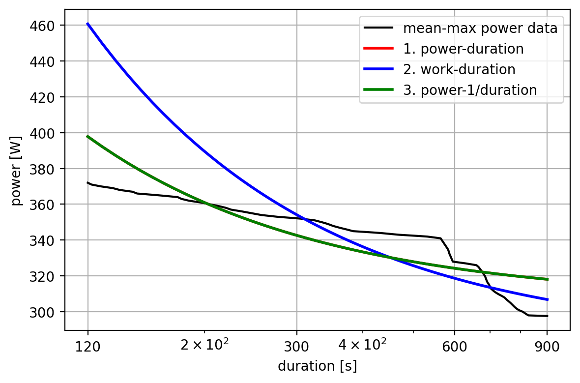
You can see that approaches 1 and 3 (power-duration and power-1/duration) completely overlap, while approach 2 (work-duration) gives different curve. The work-duration fit has a lower CP (the horizontal asymptote) but a higher W’ (which affects the curvature at shorter durations).
What I learned
Working through this helped me understand that:
The Power-Duration and Power-1/Duration approaches are mathematically identical: They’re both minimizing squared errors in power space, just using different optimization techniques (non-linear vs linear). It turns out that transforming \(P = W'/t + CP\) to plot \(P\) vs \(1/t\) doesn’t change what we’re optimizing at all.
The Work-Duration approach is genuinely different: It minimizes squared errors in work space, not power space. This means errors at longer durations get weighted more heavily (since work = power × duration). For my data, this resulted in a lower CP but higher W’ estimate.
Linear transformations can be convenient but aren’t neutral: While transforming to enable linear regression is computationally simpler, the work-duration transformation actually changes what we’re optimizing for.
Why does this matter?
Understanding these different approaches helps explain why:
- Different software might give you different \(CP\) and \(W'\) values - they might be using different fitting approaches
- Some approaches might be more appropriate depending on your use case (do you care more about accuracy at short or long durations?)
- The “same” model can produce different results depending on implementation details
The key insight for me was that while approaches 1 and 3 are truly the same thing (but dressed up differently), approach 2 is fundamentally different. It’s still fitting the \(CP\) model equation, but it’s optimizing for a different objective. The choice between them isn’t just about computational convenience, it’s about what errors you want to minimize.
The next step for me is to see how this insight can be combined with the asymmetric loss approach to see if we can get an even better fit.